Waclaw Sierpinski, a polish mathematician, and his collegues devised several curves that all bear his name. The most famous one, the Sierpinski Gasket, is dated back around 1916.
These curves are based on different geometrical basis but share the same construction principle: the Sierpinksi Gasket or Sierpinski Triangle, the Sierpinski Carpet or Sierpinski Rectangle, the Sierpinski Pentagon and the Sierpinski Hexagon.
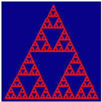
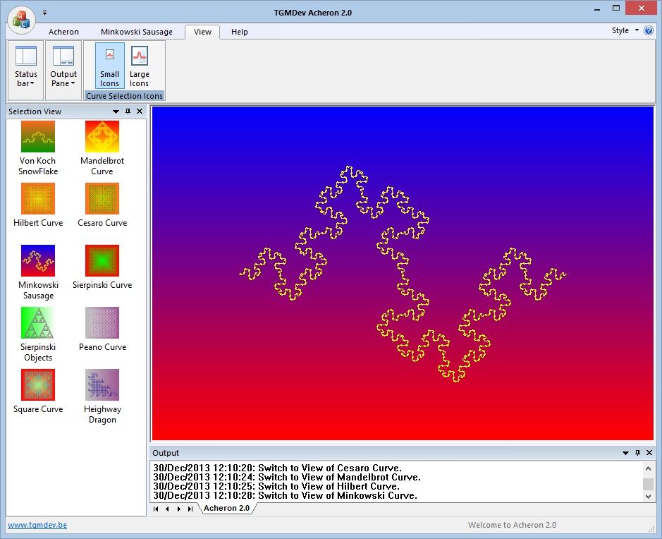
All pictures are from Acheron 2.0, a free explorer of geometrical fractals. You can download Acheron 2.0 here
Construction Back to Top
Two drawing methods are available:
- Geometric Method
- Triangle
- Rectangle
- Pentagon
- Hexagon
- Random-Based Method
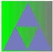
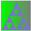
The starting point is a triangle. Divide its three sides in two segments of equal length. Connect the midpoints to get four inner triangles and paint the three external ones.
Apply the same process to the inner triangles but the middle one.
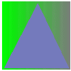
The first iterations give the following pictures:

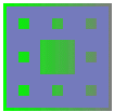
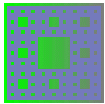
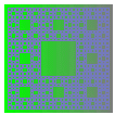
Take a rectangle. Divide the four sides in three segments of equal length. From the midpoints, drawn the lines to get the nine inner rectangles. Paint all the inner rectangles but the middle one.
Apply the same process to the inner rectangles but the middle one.
The first iterations give the following pictures ( first not shown):
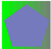
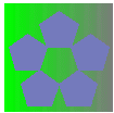
Divide a pentagon so that 6 inner pentagons can be drawn out of it. Paint all the inner pentagons but the middle one.
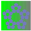
Apply the same process to the inner pentagons but the middle one.
The first iterations give the following pictures:
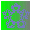
Divide an hexagon so that 6 inner hexagons can be drawn out of it. Paint all the inner hexgons. In the middle of the drawing, a star appears. Leave it unpainted.
Apply the same process to the inner hexagons.
The first iterations give the following pictures:
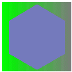
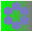
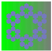
Increasing the iteration number provides more detailed drawings. However, above 6 iterations, the size of the generated inner objects becomes so small ( in fact, close to a single pixel) that further iterations are useless, only increasing the time of curve drawing.
This method is also called the Chaos Method. It works the same for all the basic figures, with the exception of the square that does not share exactly the same behaviour ( at least in my hands ...) To start drawing the Sierpinski triangle, select a vertex of the triangle. Then select randomly a second vertex and draw the point that lies in the middle of the virtual line connecting the two selected vertices. From that new point, connect a virtual line to another vertex ( selected randomly) and draw the midpoint of that line. Use that point as a start for the next iteration of the drawing process.
After a while ( say, more than one thousand iterations), a ghost curve appears, that look like the Sierpinki gasket. Then, the more points you draw, the better the curve details appears.
The curve on the left was drawn with the geometric method. On the right, the curve drawn with the chaos method.
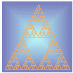
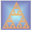
Here are the figures to get the 'midpoint' for the chaos method:
| Geometric Figure | Divider |
|---|---|
| Triangle | 2 |
| Square | 3 (*) |
| Pentagon | 2.618033 |
| Hexagon | 3 |
Note: in my hands, the chaos method gives a slightly different Sierpinski carpet. Perhaps, should I call this curve differently ...
Properties Back to Top
- Curve Length
- Curve Area
- Fractal Dimension
- Sierpinski Triangle
Replacing N by three ( as each iteration creates three self-similar triangles) and r by two ( as the sides of the triangles are divided by two) in the Hausdorff-Besicovitch equation gives:
D = log(3) / log(2) = 1.5849625
- Sierpinski Rectangle
Replacing N by 8 ( as each iteration creates eight self-similar rectangles) and r by three ( as the sides of the rectangles are divided by three) in the Hausdorff-Besicovitch equation gives:
D = log(8) / log(3) = 1.8927892
- Sierpinski Pentagon
The ratio between an inner pentagon and its parent is:
Ratio = 2 + 2 * cos(72) = 2.618033
Replacing N by 5 ( as each iteration creates fives self-similar pentagons) and r by 2.618033 ( as the ratio between pentagons from successive iteration is 2.618033) in the Hausdorff-Besicovitch equation gives:
D = log(5) / log(2.618033) = 1.6722766
- Sierpinski Hexagon
Replacing N by 6 ( as each iteration creates six self-similar hexagons) and r by 3 ( as the ratio between the sides of hexagons from successive iteration is 3) in the Hausdorff-Besicovitch equation gives:
D = log(6) / log(3) = 1.6309297
- Self-Similarity
- Link with Von Koch Curve
Intuitively, the length of the Sierpinski gasket is the total of the length of all the segments required to draw the object.
Consider the length S of the side of the starting triangle as a unit length. The perimeter of the triangle is 3S
The first iteration creates three triangles out of one, each having a side length equal to half the side length of the triangle it came from.
The total length is then equal to :
On the next iteration, each triangle gives three smaller triangles having a side length half of that of their parent, so that the total length is then equal to
Assuming a unit length S for the side of the starting triangle, we obtain the following figures:
| Iteration Number | Curve Length | Triangle Number | Curve Length |
|---|---|---|---|
| 1 | 3S | 1 | 3.00 |
| 2 | 9S ⁄2 | 3 | 4.50 |
| 3 | 27S ⁄4 | 9 | 6.75 |
| 4 | 81S ⁄8 | 27 | 10.12 |
| 5 | 243S ⁄16 | 81 | 15.19 |
| 6 | 729S ⁄32 | 243 | 22.78 |
| 7 | 2187S ⁄64 | 729 | 34.17 |
| ... | ... | ... | ... |
| 10 | 59049S ⁄512 | 19683 | 115.33 |
| n | 3nS ⁄2(n - 1) | 3(n - 1) | Tends to Infinity |
Of course, the figures at the bottom of the table does not have any physical meaning if we speak about actually drawing such a curve as there are no physical objects of that size ... but they show a really amazing property of these curves: as the number of iteration increases, the curve length tends to infinity while it is 'enclosed' in a null area !!!
First, consider the area of the first equilateral triangle as a unit area.
During the first iteration, we get 4 inner triangles, each having an area equal to one quarter of the area of the original triangle. As the middle one is left unpainted, the total area of the Sierpinski curve after the first iteration is 3/4 of the original area.
Applying the same process on each three remaining triangles, we get 9 painted triangles, each having one sixteenth of the original area. The total area is now 9/16 of the original area.
The total area can be expressed as:
Area = (3/4)n where n is the iteration number.
Here are the figures for the first iterations:
| Iteration Number |
Triangle Number |
Triangles Area |
Curve Area |
|---|---|---|---|
| 1 | 1 | 1 | 1.00 |
| 2 | 3 | 1/4 | 0.75 |
| 3 | 9 | 1/16 | 0.5625 |
| 4 | 27 | 1/64 | 0.4218 |
| 5 | 81 | 1/256 | 0.3164 |
| ... | ... | ... | ... |
| 10 | 19683 | 1/262144 | 0.0750 |
| 15 | 4782969 | 1/268435456 | 0.0178 |
| 20 | 1162261467 | 1/274877906944 | 0.0042 |
At infinite iteration, the curve area converges towards Zero, meaning that the Sierpinski gasket have no area !!! How amazing, if you remember that the curve length grows indefinitely as the number of iteration increases...
The other Sierpinski objects share the same properties, only the rate of the area decrease being different.
The fractal dimension is computed using the Hausdorff-Besicovitch equation:
D = log (N) / log ( r)
Self-similarity is one of the features exhibited by fractals that is best illustrated by the Sierpinski gasket.
Take any of the three inner triangles of a Sierpinsky gasket and magnify it twice. The curve obtained that way is similar to the whole curve it came from. This is what is called self-similarity.
On the left, the original curve. The image was then magnified twice and the top inner triangle cut out of the drawing. It is showed on the right. The small 'legs' at the bottom are the top vertices of the two lower inner triangles of the original curve.
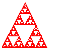
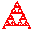
From those drawings, the self-similarity becomes self-evident ...
If you take a close look to the Siepinski hexagon, you will see that the Von Koch curve appears in the center to the drawing
If you think about the way the hexagons are drawn inside the original hexagon, that feature will start being obvious ...
All Variations described are available using Acheron 2.0
The construction of the Sierpinski Objects allows several variations.
- Drawing Method
- the geometric method
Based on basic geometry, it's a fast drawing method. - the chaos method
Based on randomness, it could take a while if you like tiny details ... - Iteration Level
- Base Geometrical Figure
Two methods are available:
See Construction for details.
This is of course a most basic variation for the drawing of the curve. Up to 8 iterations can be performed. Above this limit, the length of the different line segments comes down close to a single pixel, meaning that any increase would not yield a significantly more detailed drawing.
As explained above ( in Construction), four basic geometric figures can be used for the drawings: the triangle, the square, the pentagon and the heaxagon.
Paper Title:In situ observation of graphene sublimation and multi-layer edge reconstructions
Authors: Jian Yu Huanga,1, Feng Dingb,c, Boris I. Yakobsonc,1, Ping Lud, Liang Qie, and Ju Lie,1
Reference: http://www.pnas.org/content/early/2009/06/10/0905193106.full.pdf
Paper Title:In situ observation of graphene sublimation and multi-layer edge reconstructions
Authors: Jian Yu Huanga,1, Feng Dingb,c, Boris I. Yakobsonc,1, Ping Lud, Liang Qie, and Ju Lie,1
Reference: http://www.pnas.org/content/106/25/10103.full.pdf
Author Biography Back to Top
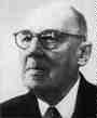 Born: 14 March 1882 in Warsaw, Poland
Died: 21 Oct 1969 in Warsaw, Poland
Waclaw Sierpinski attended school in Warsaw where his talent for mathematics was quickly spotted by his first mathematics teacher.
This was a period of Russian occupation of Poland and despite the difficulties, Sierpinski entered the Department of Mathematics and Physics of the University of Warsaw in 1899. The lectures at the University were all in Russian and the staff were entirely Russian. It is not surprising therefore that it would be the work of a Russian mathematician, one of his teachers Voronoy that first attracted Sierpinski.
In 1903 Sierpinski was awarded the gold medal for an essay on Voronoy's contribution to number theory.
Sierpinski graduated in 1904 and worked for a while as a school teacher of mathematics and physics in a girls school in Warsaw. However when the school closed because of a strike, Sierpinski decided to go to Krakov to study for his doctorate. At the Jagiellonian University in Krakov he attended lectures by Zaremba on mathematics, studying in addition astronomy and philosophy. He received his doctorate and was appointed to the University of Lvov in 1908.
When World War I began in 1914, Sierpinski and his family happened to be in Russia. When World War I ended in 1918, Sierpinski returned to Lvov. However shortly after taking up his appointment again in Lvov he was offered a post at the University of Warsaw which he accepted. In 1919 he was promoted to professor at Warsaw and he spent the rest of his life there.
Sierpinski was the author of the incredible number of 724 papers and 50 books. He retired in 1960 as professor at the University of Warsaw but he continued to give a seminar on the theory of numbers at the Polish Academy of Sciences up to 1967.
He was awarded honorary degrees from the universities Lvov (1929), St Marks of Lima (1930), Amsterdam (1931), Tarta (1931), Sofia (1939), Prague (1947), Wroclaw (1947), Lucknow (1949), and Lomonosov of Moscow (1967).
He was elected to the Geographic Society of Lima (1931), the Royal Scientific Society of Liège (1934), the Bulgarian Academy of Sciences (1936), the national Academy of Lima (1939), the Royal Society of Sciences of Naples (1939), the Accademia dei Lincei of Rome (1947), the German Academy of Science (1950), the American Academy of Sciences (1959), the Paris Academy (1960), the Royal Dutch Academy (1961), the Academy of Science of Brussels (1961), the London Mathematical Society (1964), the Romanian Academy (1965) and the Papal Academy of Sciences (1967).
Biography From School of Mathematics and Statistics - University of StAndrews, Scotland