Sierpinski Curve in Acheron 2.0

The Sierpinski curve, named from the polish mathematician Waclaw Sierpinski who originally devised it around 1912, is much less known than the other fractal objects created by Sierpinski and his co-workers as the Sierpinski gasket or the Sierpinski Carpet. However, this curve allows beautiful variations that make it a wonderful candidate for our excursion in the world of fractals ...

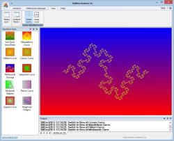
All pictures are from Acheron 2.0, a free explorer of geometrical fractals. You can download Acheron 2.0 here

As most of the fractal curves, the construction of the curve is based on the recursive procedure.

The curve grain is obtained by replacing each corner of a square by a small square placed along the diagonal axis.

The picture of the first recursion makes it easy to understand.



> This process is then repeated for the 4 corners of the figure generated at the previous iteration. The second iteration gives this picture:

The third iteration already gives an intricate pattern that require a much larger drawing to follow the construction rule visually. Playing with Acheron 2.0 will help learning the construction of this curve ...

The limit curve, obtained when iteration number tends to infinity, covers the entire area, object known as a space-filling curve.

Properties Back to Top

• Curve Length

Take a grid with a side of length N. The total length of the curve is the sum of the vertical and Horizontal segments ( noted S) and the oblique segments ( noted O).

The number of Horizontal and Vertical segments is computed using the number of segments generated at the previous recursion, the number of segments of the recursion 1 being equal to 8 ( S¹ = 8).

S^Rec = (S^Rec-1 * 4) + 8

This leads to a generalized formula for the number of Horizontal and Vertical segments:

S^Rec = ((8 * 4 ^Rec) - 8) / 3

The number of oblique segments is computed using the number of segments generated at the previous recursion, the number of segments of the recursion 1 being equal to 12 ( O¹ = 12).

O^Rec = (O^Rec-1 * 4) - 4

This leads to a generalized formula for the number of Oblique segments:

O^Rec = ((8 * 4 ^Rec) + 4) / 3

The Size of the horizontal and vertical segments changes with the recursion according to the following formula:

ls^Rec = N / (2^Rec * 4)

This is summarized in the table below:



Iteration Number	Segment Length	Horz & Vert Segments	Oblique Segments
1	N/8	8	12
2	N/16	40	44
3	N/32	168	172
4	N/64	680	684
5	N/128	2728	2732


As expected from the principe of curve construction, the ratio of the total number of segments between two successive iterations tends to 4.

Considering N being of unary length and by combining the different formula showed above, we have the following figures for the total length:



Iteration Number	Total Length of Segments		Total Curve Length
	Horz & Vert	Oblique
0	1	2.1	3.12
1	2.5	3.89	6.39
2	5.25	7.60	12.85
3	10.63	15.11	25.74
4	21.31	30.18	51.50
5	42.65	60.35	103.00
6	85.32	120.68	206.01



Roughly, the length is doubling at each iteration. Graphically, it gives:




• Curve Area

The number of full squares is equal to:

S^Rec = ((16 * 4 ^Rec) - 16) / 3

The number of half squares is equal to:

O^Rec = ((8 * 4 ^Rec) + 4) / 3

Combining these two formula gives the total number of squares:

Number^Rec = ((20 * 4 ^Rec) - 14) / 3)

To compute the total area, the total square number covered by the curve is divided by the total number of squares of the grid area:

Area^Rec = ( N * (20 * 4 ^Rec) - 14) / (3 * 4^Rec * 16))

which finally simplifies to:

Area^Rec = N * (( 10 * 4 ^Rec) - 7) / (24 * 4 ^Rec)

As the number of recursion increases, the terms 10 * 4 ^Rec and 24 * 4 ^Rec become so large that the correction by 7 have smaller and smaller influence and can be neglected. The formula tends to:

Area^Rec = N * ( 10 * 4 ^Rec) / (24 * 4 ^Rec)

which finally simplifies to:

Area^Rec = N * ( 5 / 12) = N * 0.416666

The following figures illustrates this trends:


Iteration Number	Square Number	Square Area	Curve Area
1	22	N/64	0.34175
2	102	N/256	0.39843
3	422	N/1024	0.41211
4	1702	N/4096	0.41553
5	6822	N/16384	0.41638
...	...	...	...
10	6990502	N/16777216	0.41666



The Sierpinski curve also share the very interesting property of the most fractals: its area converges rapidly to a finite limit while the total length of the segments that composed that curve have no limit.


• Fractal Dimension

The fractal dimension is computed using the Hausdorff-Besicovitch equation:

  D = log (N) / log ( r)

Replacing r by two (as on each iteration, the size of the objects is divided by two) and N by four (as the drawing process yields 4 self-similar objects) in the Hausdorff-Besicovitch equation gives:

  D = log(4) / log(2) = 2

The Box-Counting method gives the same result.



Recursion	Squares Number (N)	log(N)	Square Size (r)	log(r)
1	22	1.3424	N/8	0.9031
2	102	2.0086	N/16	1.2041
3	422	2.6253	N/32	1.5051
4	1702	3.2309	N/64	1.8062
5	6822	3.8339	N/128	2.1072
...	...	...	...
10	6990502	6.8445	N/6990502	3.6123


The plot of log(N) againts log(r) gives the following picture:


Using the figures showed in the table, the linear regression yields a slope equal to 2.0005, as expected.

A curve with a fractal dimension equal to 2 tends to cover the entire area in which it is drawn, as effectively observed when the iteration number is increased sufficiently.


• Self-Similarity

This property means that every part of the curve have the same overal character than the whole picture.

• Iteration Level

The first iterations give richer and richer drawings. Above a given level, the curve fills completely the drawing area, as all the curves with a fractal dimension equal to 2.



• Curve Style

Two ways for rendering the curve are available:


• Normal
  
  
• Filled
  
  

On both style, a grid can be added (interesting for box-counting ...)

This was a period of Russian occupation of Poland and despite the difficulties, Sierpinski entered the Department of Mathematics and Physics of the University of Warsaw in 1899. The lectures at the University were all in Russian and the staff were entirely Russian. It is not surprising therefore that it would be the work of a Russian mathematician, one of his teachers Voronoy that first attracted Sierpinski.

In 1903 Sierpinski was awarded the gold medal for an essay on Voronoy's contribution to number theory.

Sierpinski graduated in 1904 and worked for a while as a school teacher of mathematics and physics in a girls school in Warsaw. However when the school closed because of a strike, Sierpinski decided to go to Krakov to study for his doctorate. At the Jagiellonian University in Krakov he attended lectures by Zaremba on mathematics, studying in addition astronomy and philosophy. He received his doctorate and was appointed to the University of Lvov in 1908.

When World War I began in 1914, Sierpinski and his family happened to be in Russia. When World War I ended in 1918, Sierpinski returned to Lvov. However shortly after taking up his appointment again in Lvov he was offered a post at the University of Warsaw which he accepted. In 1919 he was promoted to professor at Warsaw and he spent the rest of his life there.

Sierpinski was the author of the incredible number of 724 papers and 50 books. He retired in 1960 as professor at the University of Warsaw but he continued to give a seminar on the theory of numbers at the Polish Academy of Sciences up to 1967.

He was awarded honorary degrees from the universities Lvov (1929), St Marks of Lima (1930), Amsterdam (1931), Tarta (1931), Sofia (1939), Prague (1947), Wroclaw (1947), Lucknow (1949), and Lomonosov of Moscow (1967).

He was elected to the Geographic Society of Lima (1931), the Royal Scientific Society of Liège (1934), the Bulgarian Academy of Sciences (1936), the national Academy of Lima (1939), the Royal Society of Sciences of Naples (1939), the Accademia dei Lincei of Rome (1947), the German Academy of Science (1950), the American Academy of Sciences (1959), the Paris Academy (1960), the Royal Dutch Academy (1961), the Academy of Science of Brussels (1961), the London Mathematical Society (1964), the Romanian Academy (1965) and the Papal Academy of Sciences (1967).

Biography From School of Mathematics and Statistics - University of StAndrews, Scotland